
During the course of a NetEye installation, a wide range of performance data is collected. From latency metrics of ping checks, to the saturation data of disks and memory units, to the collection of utilization metrics of various kinds. For all of this data we’ve adopted the open source time series database InfluxDB.
The time-aligned method of allocating data makes InfluxDB a great choice for comparing data from various sources over a specific time frame. Just such a use case arose during a recent project in the context of an IoT environment, where we wanted to collect performance data from a large number of devices. Given that the number of devices was only expected to grow, the customer desired to keep historical data for a period of at least one year.
Since the IoT data is collected at a resolution rate of 10 seconds, the quantity of stored performance data grows quite quickly. This was the point at which we asked ourselves whether we actually need to keep all that data at such a high resolution for such a long period of time.
We decided to implement a retention management policy to keep only very recent data at full resolution. Data older than one month would instead be kept as a single aggregated average data point per hour.
In order to realize this concept, we chose an implementation path using continuous queries and retention policies. To give a rough understanding of both concepts, I suggest you read about the principles behind a retention policy and how to implement the concept of downsampling, combining retention policies and continuous queries in InfluxDB.
Retention Policy Management
Based on the concepts of defining retention policies, we decided to limit the default retention policy to 1 month, while adding an additional retention policy to store the lower resolution data for 1 year. This latter retention policy represents all data collected for 1 year at the resolution of 1 data point per hour.
For this we first start by implementing a new retention policy acting in addition to the default “autogenerated” retention policy. We create this retention policy with a duration of 365 days:
> CREATE RETENTION POLICY rp_365d ON perfdata DURATION 365d REPLICATION 1
> ALTER RETENTION POLICY "autogen" ON "perfdata" DURATION 30d SHARD DURATION 2h DEFAULT

> show retention policies
name    duration  shardGroupDuration replicaN default
----    --------  ------------------ -------- -------
autogen 720h0m0s  2h0m0s             1        true
rp_365d 8760h0m0s 168h0m0s           1        false
Continuous Queries
Now we have another retention policy within the same database, but data is still collected only within the “autogen” retention policy. Here continuous queries come into play: They ship the downsampled performance data into the new retention policy.
We start with the definition of a create continuous query statement and define it to read the mean() of the “value” of all fields for 1 hour from all measurements available in the current database, and then write it into the new retention policy “rp_365d” while maintaining the name of the original measurement.
HINT: If you omit the “AS value” in the Select section, the newly created field will be named “mean_value” instead of retaining the name “value”. If you don’t do so, visualization in Grafana will be more difficult.
CREATE CONTINUOUS QUERY "cq_measurementXX" ON "measurementXX"
BEGIN
   SELECT mean(value) AS value
   INTO "perfdata"."rp_365d".:MEASUREMENT
   FROM /.*/
   GROUP BY time(60m),*
END
Creating Visualizations in Grafana that Adapt Dynamically to a Suitable Retention Policy
We now have performance data collected in InfluxDB according to our two retention policies. Visualization in Grafana should adapt according those retention policies.
Unfortunately, the behavior is not that automatic, and the select statements within the various visualizations act on a specific retention policy (if not specified, they default to “autogen”). But we wanted to see performance data at the highest resolution whenever we are observing data from the most recent 30 days!
In the Grafana user forum I found a rather interesting discussion about implementing dynamic visualization in Grafana: https://github.com/grafana/grafana/issues/4262
Here I’ll explain the approach to you with a simple example:
Step 1: Map your retention policies through 2 data series stored within a single dedicated retention policy:
CREATE RETENTION POLICY "forever" ON perfdata DURATION INF REPLICATION 1
Step 2: For each retention policy, write a series indicating the start and end times of the corresponding retention policy:
INSERT INTO forever rp_config,idx=1 rp="autogen",start=0i,end=2592000000i -9223372036854775806 INSERT INTO forever rp_config,idx=2 rp="rp_365d",start=2592000000i,end=31536000000i -9223372036854775806
Note: I assumed a day length of 86400000. Insert #1 is that value × 30, and Insert #2 is × 365.
Now verify the stored data:
select * from forever.rp_config
   name: rp_config
   time                 end        idx rp      start
   ----                 ---        --- --      -----
   -9223372036854775806 2592000000 1   autogen 0
   -9223372036854775806 3153600000 2   rp_365d 2592000000
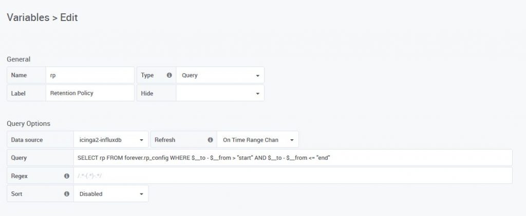
Next, create a “variable” in Grafana that provides you with the suitable retention policy for the chosen time frame:
Variable name: rp
Type: Query
Query: SELECT rp FROM forever.rp_config WHERE $__to - $__from > "start" AND $__to - $__from <= "end"
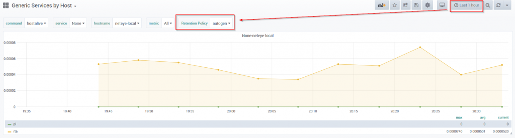
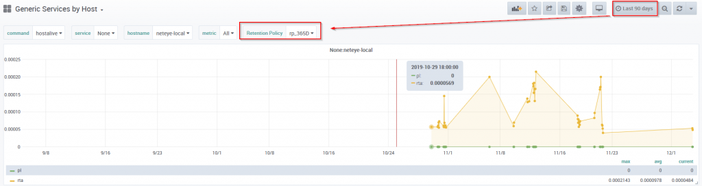
And now, apply this variable to the queries for your Grafana graphs and look at the results:
- When visualizing the time range now – “last 30 days”, the “autogen” retention policy is automatically selected
- When visualizing the time range “last 30 days” to “last 365 days” the retention period “rp_365d” is chosen.


Hallo.
I tried to execute your configuration step by step bu I obtained error when I tried to insert a series:
> INSERT INTO forever rp_config,idx=1 rp=”DATI_SETTE_GIORNI”,start=0i,end=604800000i -9223372036854775806
ERR: {“error”:”unable to parse ‘rp_config,idx=1 rp=\”DATI_SETTE_GIORNI\”,start=0i,end=604800000i -9223372036854775806’: invalid boolean”}
Could you help me?
Thanks a lot
Mario
Hello Mario,
this error could derive from an encoding error. Maybe the conversion into Boolean fails because of special characters when copy from web is done. Can you try to convert the insert statement into pure ASCII by copy-paste from a text editor like notepad++ ?
In addition you can follow the example shown in github issue https://github.com/grafana/grafana/issues/4262. My choosen approach had been discussed within this issue.
Kind regards,
Patrick
Hi, I have followed your guide, but my rp_365d retention policy keeps data just for a month (same as autogen). the rp duration is correct, downsampling is working, but the oldest shard of rp_365d starts on the same date autogen shard. Can you help how to correct it?