30. 06. 2026
APM, DevOps, Kubernetes

19. 09. 2022
Davide Sbetti
Log-SIEM, Machine Learning
Elasticsearch ML Models and Inference: Real-Time Classification
In a previous article, we explored the Machine Learning capabilities of Elasticsearch, which allowed us to apply anomaly detection techniques to our data, and helped us discover some really interesting facts as a result of our analysis.
But can we take that idea even further? For instance, could we use data we’ve already collected to enrich new incoming data points in real-time?
As you might imagine, the answer to all these questions is: absolutely yes!
Data Frame Analytics: Training a Model
Elasticsearch offers the possibility of training a model through its Data Frame Analytics functionality, accessible from the Machine Learning section.
Our data and goal
In our scenario, we are using NetEye to monitor a set of high-frequency antennas with the goal of identifying free electrons in the ionosphere, namely the upper section of our atmosphere, to aid scientific research.
The scientists working on this research project have already labeled some of the received signals as belonging to one the following two classes:
- Good radar signals: signals returning information about certain structures in the ionosphere, namely the target of the research
- Bad radar signals: signals passing through the ionosphere without encountering any particular electron-based structure.
We can import the labeled data, which is both attached here in this article (in a slightly modified format and with one data point being removed for later use) and also available from the UCI Machine Learning Repository, by uploading the file directly to Elasticsearch.
From the index we created, we can observe that each signal is composed of 34 numeric values (renamed for simplicity in the attached dataset as attribute1 … attribute34. Moreover, each signal also contains the class assigned by one of the scientists in its class attribute.
So now can we give our scientists some more free time by automatically recognizing whether the signal collected by our antennas is good or bad?
We can… we just have to build a classification model that automatically recognizes the type of a newly collected signal data point!
Supervised Learning vs Unsupervised Learning
I promise the boring part here will be short. We just need to analyze the problem we just defined in more detail to understand how this can be solved. Generally, machine learning models are trained according to one of the following two methods:
- Supervised learning: Also known as learning by example, this is similar to how we would teach a child to distinguish between, say, Formula 1 sport cars and sedans. For instance, we could take a set of toy cars and start dividing them into two sets as the child watches. Soon, he/she will understand which characteristics to look at when distinguishing sport cars from sedans, such as the more aerodynamic shape of sport cars.
Training models with the supervised learning method works in a similar way. The basis is a dataset that contains data points which already include the attribute we would like to predict. The target attribute can be a number (a regression task) or a categorical value (a classification task). - Unsupervised learning: As you can imagine, this is the opposite case, where the data is not already “labeled”. The algorithm will thus base its model only on the characteristics of the data itself as it was collected, without any human intervention.
Two examples of unsupervised learning applications include outlier detection (finding anomalies) and clustering (automatically creating new groupings based on the characteristics of the data). If we give an unsupervised algorithm our same set of cars as above, it might give us back light colored cars vs. dark ones, or tall cars vs. short cars, depending on the relationships it finds by itself in the data.
Building a Classification Model in Elastic
Now that we’ve learned the differences in how the models are trained, we can now recognize when we are in a supervised learning scenario, and and aiming to build a classification model.
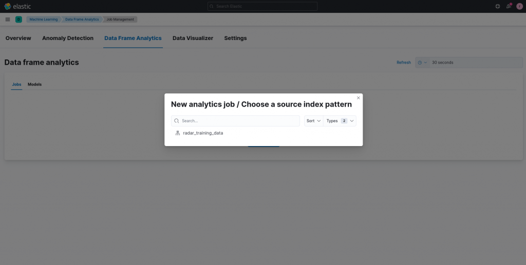
So let’s open the Data Frame Analytics module and create a new training job based on the data we imported previously.
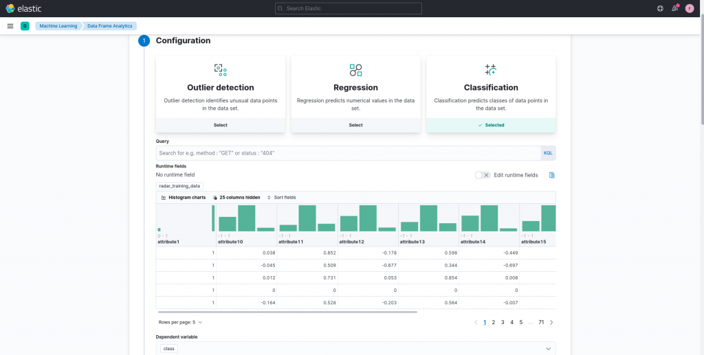
On the job configuration page, we can select classification as goal of our model. The next step is to select the dependent variable(s), so the target attribute we would like to predict, which in the case of the attached dataset is the class attribute.
We can now personalize the set of fields that we would like to consider for the prediction. In our case, since we are not domain experts (at least, I am definitely not), we can include them all, leaving it up to the model to determine which are important and which are not.
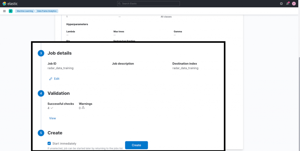
Furthermore, we can specify the training/test percentage. What does this mean? Basically, a certain percentage of data points will not be used for training the model, but will instead be used to evaluate its predicting capabilities after the training phase is completed. This avoids testing a model on data it has already seen during the training phase, which can lead you to think that your model is better than it actually is. We can keep the standard 80/20 ratio (80% training, 20% testing) for our example model.
Moreover, we can now configure some hyperparameters, namely parameters used by the training algorithm itself independent of any data, which, in the case of classification in Elasticsearch turns out to be decision trees. When training our example model, I didn’t change this configuration.
And now we can choose a name for our job and start training!
The Resulting Model
Once the training procedure is completed, we can consult the model evaluation report by clicking on the View Results button. This, in the case of the classification model, shows what’s generally known as a confusion matrix. The matrix reports, for our two classes, the percentage of data points that were both classified correctly and those misclassified. We can view the matrix for the entire dataset or just the training or testing subsets individually.
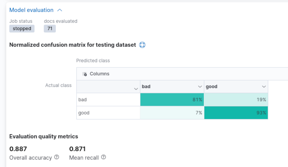
We can observe that our model performed reasonably well, especially given that we did not investigate any particular technique to boost its capabilities.
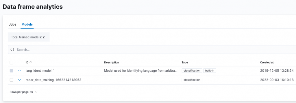
The trained model is then shown in the models list, under the Data Frame Analytics section. Please note the ID of the model, since we’ll use it later.
So, how do we apply our trained model to future unclassified data points?
Inference
Now that we have a classification model ready to be used on future data points, all we need is the Inference processor. This processor can be added to an Ingest Pipeline, and allows us to apply an already trained model to new, incoming data points.
To do that we add a new pipeline under the Ingest Pipelines setting of the Stack Management UI.
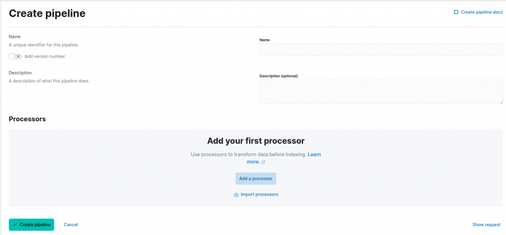
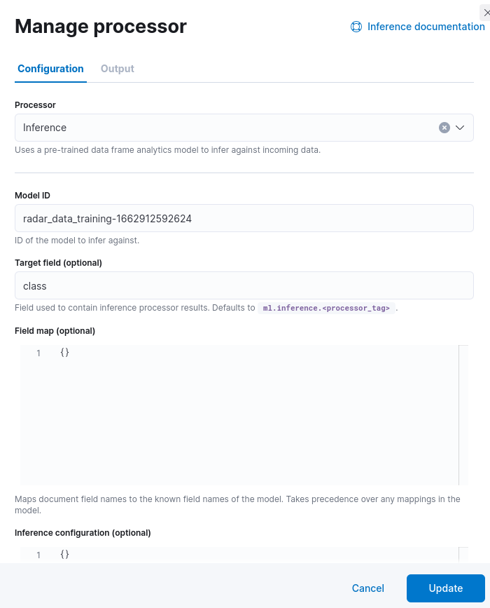
We can now specify a name for our pipeline and add a processor. From the available list, choose the Inference processor. When configuring the processor, we must set (1) the model ID we noted during the previous step and optionally specify the target field, (2) the field which will contain the result of our classification, and (3) a field mapping, in case the incoming data points are stored in a different format.
In our case, we can specify the class attribute to host the model classification, similar to the data points used during training, and we don’t need to specify any new mapping for the fields. Furthermore, we also don’t customize the settings related to the inference processor itself, for which a more detailed description is available in the official documentation.
Before creating the pipeline, we can test it by using the option available in the UI. Let’s use the following data point, which was removed from the original data set, to test that our pipeline is functioning correctly:
[
{
"_source": {
"attribute1": 1,
"attribute2": 0,
"attribute3": 0.84710,
"attribute4": 0.13533,
"attribute5": 0.73638,
"attribute6": -0.06151,
"attribute7": 0.87873,
"attribute8": 0.08260,
"attribute9": 0.88928,
"attribute10": -0.09139,
"attribute11": 0.78735,
"attribute12": 0.06678,
"attribute13": 0.80668,
"attribute14": -0.00351,
"attribute15": 0.79262,
"attribute16": -0.01054,
"attribute17": 0.85764,
"attribute18": -0.04569,
"attribute19": 0.87170,
"attribute20": -0.03515,
"attribute21": 0.81722,
"attribute22": -0.09490,
"attribute23": 0.71002,
"attribute24": 0.04394,
"attribute25": 0.86467,
"attribute26": -0.15114,
"attribute27": 0.81147,
"attribute28": -0.04822,
"attribute29": 0.78207,
"attribute30": -0.00703,
"attribute31": 0.75747,
"attribute32": -0.06678,
"attribute33": 0.85764,
"attribute34": -0.06151
}
}
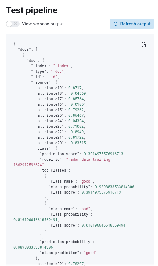
]A click on the Run the pipeline button will show us the output of the pipeline. As you can see from the image below, among the various attributes we can now find the class attribute, which contains the predicted probability for both our target classes and, under the class_prediction attribute, the one with the largest probability.
Having successfully tested our pipeline, we can proceed to finalizing it.
Applying our Predictive Ingest Pipeline
In order to apply our predictive ingest pipeline, we can create an index template matching a specific pattern, in our case radar-collected-data-*. In the template’s configuration we set as the final pipeline our ingest pipeline name we specified earlier during pipeline creation:
{
  "final_pipeline": "radar_data_pipeline"
}
After creating the template, we can add the same document we used before during the pipeline test to an index, matching the index pattern chosen during the index template creation, by running the following query in the Console available inside Dev Tools:
PUT radar-collected-data-000001/_doc/1
{
"attribute1": 1,
"attribute2": 0,
"attribute3": 0.84710,
"attribute4": 0.13533,
"attribute5": 0.73638,
"attribute6": -0.06151,
"attribute7": 0.87873,
"attribute8": 0.08260,
"attribute9": 0.88928,
"attribute10": -0.09139,
"attribute11": 0.78735,
"attribute12": 0.06678,
"attribute13": 0.80668,
"attribute14": -0.00351,
"attribute15": 0.79262,
"attribute16": -0.01054,
"attribute17": 0.85764,
"attribute18": -0.04569,
"attribute19": 0.87170,
"attribute20": -0.03515,
"attribute21": 0.81722,
"attribute22": -0.09490,
"attribute23": 0.71002,
"attribute24": 0.04394,
"attribute25": 0.86467,
"attribute26": -0.15114,
"attribute27": 0.81147,
"attribute28": -0.04822,
"attribute29": 0.78207,
"attribute30": -0.00703,
"attribute31": 0.75747,
"attribute32": -0.06678,
"attribute33": 0.85764,
"attribute34": -0.06151
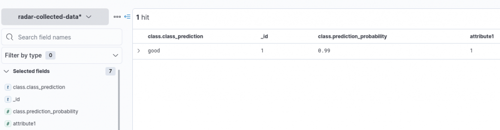
}The target index will be created and the document then successfully added. We can now add our index pattern to the ones used by Kibana under the Index patterns view inside the Stack Management option, inspecting it then via the Discover functionality. As shown in the image below, we can see how the Ingest Pipeline previously defined was applied, leading to a prediction of the class of the added document.
Conclusions
In this article, we explored how we can use Elasticsearch to train a machine learning model, starting from some training data, then applying the Inference processor inside an Ingest Pipeline to the data in future documents matching a particular index pattern.
References
Ionosphere Data Set: Blake, C., Keogh,E and Merz, C.J. (1998). UCI Repository of machine learning databases [https://archive.ics.uci.edu/ml/index.php]. Irvine, CA: University of California, Department of Information and Computer Science
Dataset
These Solutions are Engineered by Humans
Are you passionate about performance metrics or other modern IT challenges? Do you have the experience to drive solutions like the one above? Our customers often present us with problems that need customized solutions. In fact, we’re currently hiring for roles just like this as well as other roles here at Würth Phoenix.
Davide Sbetti
Hi! I'm Davide and I'm a Software Developer with the R&D Team in the "IT System & Service Management Solutions" group here at Würth IT Italy. IT has been a passion for me ever since I was a child, and so the direction of my studies was...never in any doubt! Lately, my interests have focused in particular on data science techniques and the training of machine learning models.
Author
Latest posts by Davide Sbetti
30. 06. 2026
AI, Kubernetes
Load-balancing Requests to LLMs in Kubernetes: A KV-cache Approach with llm-d!
30. 03. 2026
APM, Log Management, Log-SIEM, NetEye
Sending OTel Data to Elasticsearch: Tenant Segregation through OAuth