15. 06. 2026
NetEye, Unified Monitoring

21. 06. 2022
Davide Sbetti
Log Management, Log-SIEM
Elastic Transformations: How to Aggregate and Enrich Your Data
In a previous article I analyzed how you can create effective visualizations in Kibana, and how to apply machine learning jobs with the goal of extracting as much information as possible from our data.
However, you can also think of data as a raw material, which sometimes needs to be transformed and manipulated before allowing us to extract all possible information.
In this article, let us try to analyze some generated logs and, supposing we don’t have any particular prior knowledge, trying to understand how even simple data transformations can help us in our task.
Importing the sample data
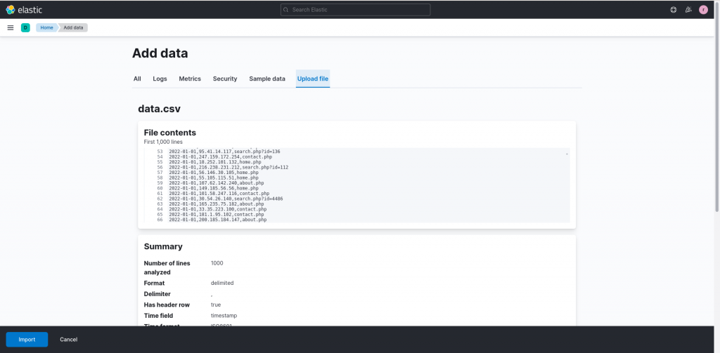
To explore the various techniques on some data, I used a Python script to generate some web logs,with some specific characteristics that we will try to uncover during our data analysis. The data, available as a .csv file attached to the end of this article, can be imported directly into the Kibana interface by clicking on Add your data and then Upload file. You can then directly drag and drop the data file to load it. A click on Import then allows us to specify the destination index and complete the loading process.
What are we looking at? A first analysis
After the upload and index creation process are completed, we can browse the data through the Discover functionality to get a first look at the characteristics of the uploaded logs.
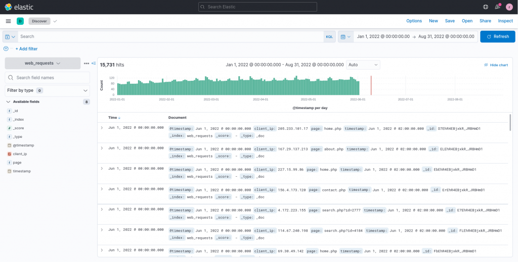
From this first look we can observe that the index contains about 16.000 web logs, although just a handful of fields, namely the timestamp of the request, the source IP (clientip) and the page visited. As also described in the previous article about data visualization, a simple plot can often help during the first phases of data analysis to understand how to proceed.
We can thus again exploit the Data Visualizer, available in the Machine Learning section, to obtain some useful initial insights.
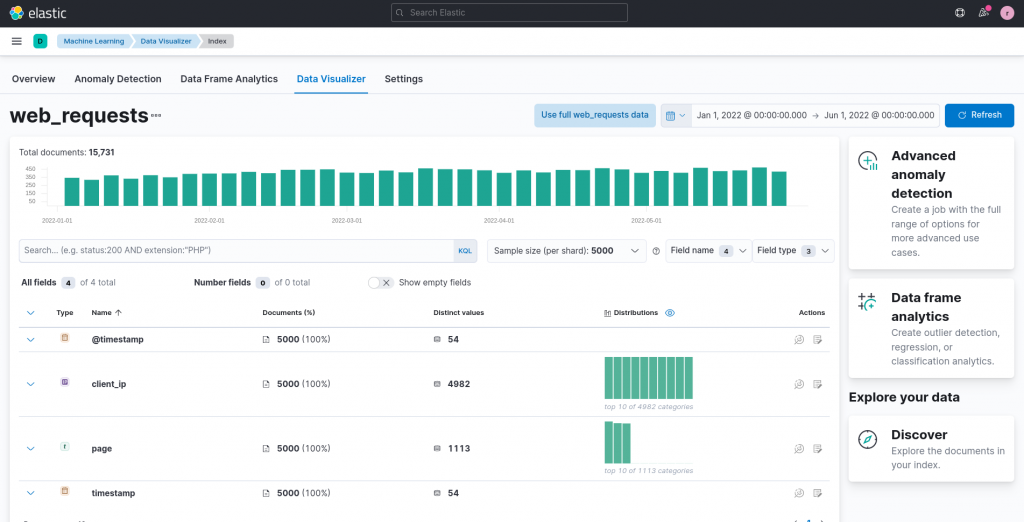
From the summary table and statistics provided by Kibana we can already tease out some characteristics from our data, taken from a sample of 5,000 logs. For example, we can see how there are understandably multiple requests per day by looking at the number of distinct values for the timestamp column. Moreover, we can also recognize in general how a single clientIP performs just a handful requests, and that thus an analysis of the traffic per IP would probably not bring us any great discoveries (in fact, this was a planned characteristic of the dataset to avoid misleading the user during the analysis).
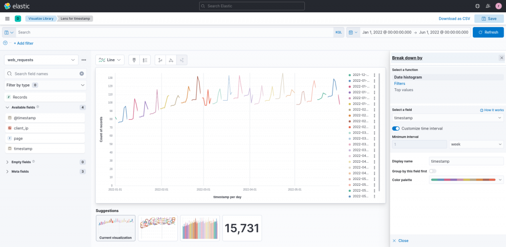
Having discovered some basic characteristics in the data we are analyzing, let’s try a first plot by analyzing the timestamp field of the requests in Lens, through the associated Action Button on the right side of its row.
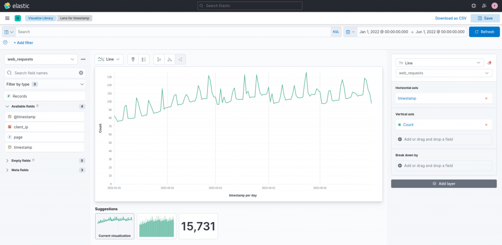
The first plot, related to the timestamp field that is generated by Lens, groups the requests per day by default, providing us with a good overall view of the requests trend.
This way we can observe how there is a slowly growing trend overall, namely the number of requests per day is growing day by day, although not rapidly. What’s also interesting to note are the repeated peaks that we can observe. Some of them, especially the lower ones, could just be noise, in other words an abnormal temporary behavior which may be caused (for instance, think about a website) by a special period/day, such as a holiday. However, some of the high repeated peaks could be the hint of a more constant distinctive behavior, which we should investigate further.
Requests on a weekly basis
Currently, the timestamps are depicted on a daily basis. However, this does not simplify the understanding of patterns on a multiple-days basis. Let’s try to break down the time series over, for example, a weekly basis. The Break down by Lens option is ideal for this purpose.
We can select the timestamp field and, by customizing the time interval in the settings panel, break down the series on, for example, a 1 week basis.
The updated plot now displays each week in a different color, and this provides us with information to refine our data exploration: we can find at least one peak in each week and, moreover, the peaks seem to always appear near the end of the week.
How can we investigate this hypothesis even further?
Data transformation
Elastic data transformations lets us define some aggregations and transformations that we can apply to our data, a process that applies not only to past data but that can also be kept running (in the so called continuous mode) for new, incoming data points.
Let’s take a look at how transformations work by accessing them under Management -> Stack Management -> Data -> Transforms.
We can create our data transformation by clicking on Create your first transform and selecting the index that contains our web requests logs. The main configuration of the transform is then displayed on the page:
In our case, we can apply the following two operations to our data:
- To understand which days are responsible for the peaks, aggregate the web requests by day (since we are interested in daily related patterns). This aggregation can also be done directly in the plot using Lens, but having a day-based index may help us perform even more analyses and more easily consult the aggregated data.
- To explore more in depth our hypothesis of the peak occurring at the end of the week (and also obtain some information on the days involved), create a new field that contains the day of the week (Monday to Sunday) in addition to the timestamp.
While aggregation comes built-in with the Pivot transformation, to achieve the second goal we can create… a runtime field!
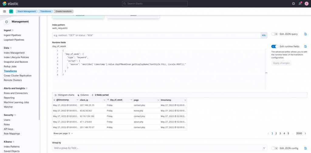
A runtime field can be used to add a field that’s not present in the original data. This operation can be performed not only during transforms, but also during queries. In our case, however, we can exploit their presence during transforms by clicking on the toggle Edit runtime fields and applying the following transformation:
{
  "day_of_week": {
    "type": "keyword",
    "script": {
      "source": "emit(doc['timestamp'].value.dayOfWeekEnum.getDisplayName(TextStyle.FULL, Locale.ROOT));"
    }
  }
}
This transform creates a new field, named day_of_week of type keyword, containing the day of week, extracted from the timestamp column, visualized according to the current locale of the user. A click on Apply changes allows us to observe a preview of the result on some sample rows.
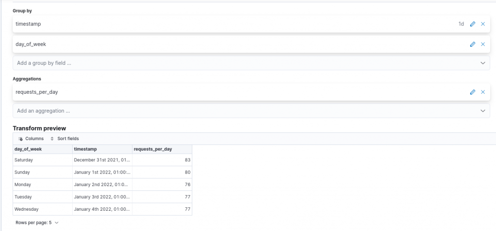
Once we are satisfied with the result of our runtime field, we can then proceed by mapping the aggregation we would like to perform. In our case, we would like to aggregate the requests per day, so we set the timestamp field as a group by field, and customizing the time interval to one day by clicking on the edit button at the end of the added field.
Moreover, since we would like to preserve the runtime field after aggregation, we must also add it as a group by field. For the aggregation, we should choose the value count aggregation for the timestamp field to reflect our goal. The name of the field resulting from the aggregation can also be customized, for example, to requests_per_day.
Clicking on Next allows us to specify the overall details of the transform, such as its ID, Kibana destination index, and whether we would like the process to also be applied to future data points. In our case this is not necessary, since the data were loaded statically from a sample data file. A second click on Next and then on Creates and start completes the transform.
Transform visualization
After having created the transform and resulting index, we can return to the Data Visualizer tool. Visualizing the field resulting from the aggregation in Lens, requests_per_day returns the same visualization we were previously only able to build with the capabilities of Lens.
However this time, we can apply a more focused break down by filter, to see the top values of the day_of_week field, focusing on the first top three values.
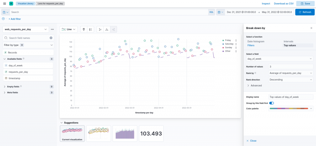
The resulting visualization precisely confirms our hypothesis, namely of the peak in requests being always near the weekend, and in particular on Fridays and Saturdays. This is likely a sign that our imaginary website is used most often right before the weekend, such as planning weekends activities or hikes.
Conclusions
In this article I explored how we can use transforms and runtime fields to aggregate and enrich our data, enabling us to more easily discover their characteristics. In particular, starting from a simple visualization of some data points, without having any prior knowledge, we applied a transformation to aggregate the given data, obtaining a “zoomed out”, high level picture. We also created a runtime field to extract information that was not explicitly present in the original index and that, used in a second visualization, reinforced our hypothesis on the characteristics of the data.
Attachments
These Solutions are Engineered by Humans
Are you passionate about performance metrics or other modern IT challenges? Do you have the experience to drive solutions like the one above? Our customers often present us with problems that need customized solutions. In fact, we’re currently hiring for roles like this as well as other roles here at Würth Phoenix.
Davide Sbetti
Hi! I'm Davide and I'm a Software Developer with the R&D Team in the "IT System & Service Management Solutions" group here at Würth IT Italy. IT has been a passion for me ever since I was a child, and so the direction of my studies was...never in any doubt! Lately, my interests have focused in particular on data science techniques and the training of machine learning models.
Author
Latest posts by Davide Sbetti
30. 03. 2026
APM, Log Management, Log-SIEM, NetEye
Sending OTel Data to Elasticsearch: Tenant Segregation through OAuth