In my previous post, we saw how it’s possible to build a simple Grafana Data Source Plugin, which we can use to read data from whatever source we’d like to use. In particular, we used it to read data from a simple web service we created so we could expose data containing some outliers.

In this post, we’ll continue that task by adding some simple outlier detection capabilities to our Data Source Plugin.

Note: All the code discussed in this blog post is available, in its final version, in a GitHub repository.

Why We Like Forests

As we all know, forests are really important for our environment! They help fight climate change by capturing carbon dioxide, they’re the home of many animal species, and they provide food and material. But, in a quite interesting way, they help us find outliers. You weren’t expecting that, were you?

Okay, in this case, we are not really talking about forests of trees as you find them in nature. Honestly, in this case we should think more along the lines of Isolation Forests!

Isolation Forests

Isolation Forests are an unsupervised machine learning algorithm, so as you might remember from a past discussion, this means that the data that we use as input for the algorithm must not already be labeled, and the model will only work on the characteristics of the data it sees, without taking into account any additional information.

Usually when dealing with anomaly detection, the main approach consists of establishing what’s “normal”, and then labeling as an anomaly everything that cannot be classified as normal.

Well, Isolation Forests work in exactly the opposite way. They try to directly detect anomalies, without “caring” about what is considered normal. How?

Intuitively speaking, the main idea behind Isolation Forests is that generally, anomalies are easier to distinguish than normal data points, because they have something different than normal points.

A Forest of what?

Okay, so we’ll use an Isolation Forest. But a forest of what? Of Decision Trees of course!

A Decision Tree is a supervised algorithm that is used both for classification and regression tasks. To understand this more easily, let’s imagine a classification task, where we’d like to understand what the rules are behind the division of a data set into some categories.

In a decision tree, everything starts from the root node, which will hold the entire data set. Then, based on certain criteria, the data set is split into two or more subsets (if we fix the number of subsets to be always two then we are talking about a Binary Decision Tree). And we continue like this until all data are completely divided into the desired categories, namely until each leaf node of the tree contains only data belonging to a certain category.

For example, let’s consider this small data set containing data about some days in which I went out for a run, and some I didn’t go, together with information about the weather conditions on that day (yes, I know… If I were a real runner I would run during all possible weather conditions.. please don’t judge me).

Outlook	Temperature	Humidity	Windy?	Did I run?
sunny	hot	high	TRUE	NO
overcast	hot	high	FALSE	YES
rainy	mild	high	FALSE	YES
rainy	cool	normal	FALSE	YES
rainy	cool	normal	TRUE	NO
overcast	cool	normal	TRUE	YES
sunny	mild	high	FALSE	NO
sunny	cool	normal	FALSE	YES
rainy	mild	normal	FALSE	YES
sunny	mild	normal	TRUE	YES
overcast	mild	high	TRUE	YES
overcast	hot	normal	FALSE	YES
rainy	mild	high	TRUE	NO

If we were to generate a decision tree out of the above data set, in order to understand how I base my decisions about going out for a run, we’ll end up with something similar to the tree below.

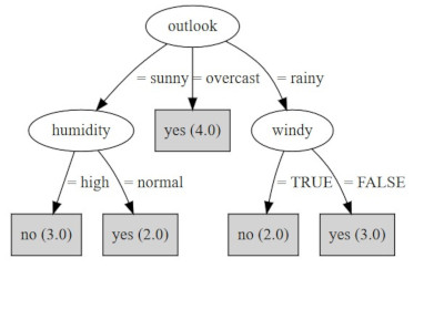
As you can imagine, the core aspect is deciding which attribute we would like to use, at each step, to divide our data into subsets. Well, without going into too much detail, let me tell you that there are various criteria that could be used for that, such as the Gini Index or the Information Gain. What they have in common, which is in the end the core idea we are interested in, is that they give us an idea of the impurity of a data set. The goal, as you can imagine, is to find at each step that one attribute that helps us most to reduce the impurity of the resulting subsets.

And yes, numerical attributes can also be used with decision trees. In this case, multiple split points are evaluated at each step, based on the chosen algorithm.

Isolation Forests for outlier detection

Okay, we now know what are decision trees and that they are the main component of Isolation Forests.

We’re all set, right?

Pausing to think about it, I can see an issue here. We mentioned that Isolation Forests are an unsupervised algorithm… while decision trees are supervised! Where’s the trick then?

The trick is in the way Isolation Forests use decision trees.

With the Isolation Forests approach, multiple decision trees are created out of the same data set, and, at each step, an attribute is randomly chosen for the split, together with a randomly chosen split point. And this is repeated until all points are isolated in a leaf node, namely, we managed to distinguish every point from the others, based on a certain combination of characteristics. Why does this help? The idea is that, since anomalies are easier to distinguish, the path in the tree that will lead to them will be shorter since fewer characteristics need to be evaluated to distinguish them from other points. And this will happen even if we choose the attributes in a random way and we repeat the process many times, afterwards analyzing the global results. If you would like to go deeper into the topic of Isolation Forests, I would suggest reading this paper.

Implementing our Grafana Data Source Plugin

Okay, we’ve had the necessary overview of the technique that we would like to use in our Grafana Data Source Plugin. Now it’s time to go back to the code.

First of all, since we don’t like re-inventing the wheel, let’s use a library that contains an implementation of the algorithm we discussed above, such as this one.

We can add it to the package.json of our plugin, which will look as follows:

...
"dependencies": {
    "@emotion/css": "^11.1.3",
    "@grafana/data": "9.2.5",
    "@grafana/runtime": "9.2.5",
    "@grafana/ui": "9.2.5",
    "debounce-promise": "3.1.2",
    "isolation-forest": "^0.0.9",
    "react": "17.0.2",
    "react-dom": "17.0.2",
    "yarn": "^1.22.19"
  }
...

We can then run yarn install to ensure the new dependency is downloaded.

After that, it’s time to move to the datasource.ts file. We can start by importing the new library:

import { IsolationForest } from 'isolation-forest'

We can then modify the query function we implemented in the previous post. Before, we were creating a result data frame containing just the time and value, and we were pushing a new point for each point that was returned by the Data Source. This time, we can add a new property in the result data frame, namely the Outlier property. We can then collect all the points returned by the Data Source, apply the Isolation Forest technique through the getOutlierLabels function, and return the original point and the label in the result data frame. The resulting function will look similar to the following one:

  async query(options: DataQueryRequest<DataQuery>): 
    Promise<DataQueryResponse> {
    
    // Extract the time range
    const {range} = options;
    const from = range!.from.valueOf();
    const to = range!.to.valueOf();

    // Map each query to a requests
    const promises = options.targets.map((query) =>
        this.doRequest(query, from, to).then((response) => {
          // Create result data frame
          const frame = new MutableDataFrame({
            refId: query.refId,
            fields: [
              {name: "Time", type: FieldType.time},
              {name: "Value", type: FieldType.number},
              {name: "Outlier", type: FieldType.boolean },
            ],
          });

          // Let's store the original points
          // returned by the data source
          let full_points: Point[] = [];

          response.data.query_response.forEach((point: any) => {
            full_points.push({time: point[0], value: point[1]});
          });

          // Get the labels, one for each point
          const outlierLabels = 
            this.getOutlierLabels(full_points);

          // Store the points and labels in 
          // the resulting data frame
          for (let i = 0; i  < full_points.length;  i++) {
            frame.appendRow([
               full_points[i].time,
               full_points[i].value,
               outlierLabels[i]
            ]);
          }
          // Return it!
          return frame;
        })
    );
    return Promise.all(promises).then((data) => ({ data }));
  }

And now… let’s get the labels! We can create an Isolation Forest using the aforementioned library. This will automatically generate about 100 decision trees, a value that was understood to be quite good for detecting anomalies. It will then return, for each point, a score between 0 and 1. As you can imagine, the closer a point’s score is to 1, the more it can be considered an anomaly (it is a real anomaly score).

For now, let’s start by keeping it simple and return a true/false value if the anomaly score is greater than 0.6, just to exclude the more “borderline” points with a score close to 0.5.

  getOutlierLabels(full_points: Point[]) {

    // Create the Isolation Forest object
    const isolation_forest = new IsolationForest();

    // Feed it with our points
    isolation_forest.fit(full_points);

    // Get back the anomaly scores
    const scores = isolation_forest.scores();

    // Let's store the true/false labels
    let outlier_labels = [];

    // Where a point is considered as anomaly if
    // the anomaly score > 0.6
    for (const score of scores) {
      if (score > 0.6) {
        outlier_labels.push(true);
      } else {
        outlier_labels.push(false);
      }
    }
    // Return the labels
    return outlier_labels;
  }

Time to Check the Results: a Grafana Dashboard

Now that we’ve implemented a simple mechanism to find outliers, it’s time to test it!

Let’s start by deploying the Data Source Plugin by executing the build_and_apply.sh script, available in the repository.

We can then launch the webserver exposing the data using flask run as we saw last time, and we can create, if it doesn’t yet exist, a Grafana Data Source pointing to our plugin.

We can then create a simple dashboard, such as the one you can find in the dashboard folder of the repository, to test our plugin (if you’d like to upload the provided dashboard, just remember to change the Data Source to the one you created on your Grafana instance).

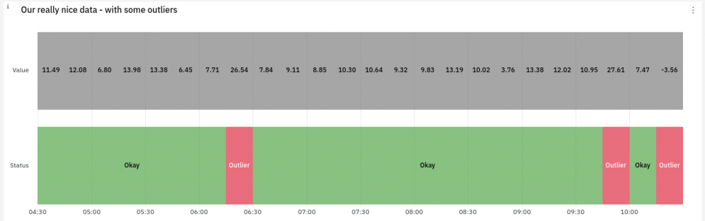
For example, we can use the State Timeline panel to display a nice timeline where outliers are clearly marked. Moreover, by applying a custom Value Mapping, we can associate arbitrary labels (such as “Okay” and “Outlier”) and colors (green/red) to the boolean field we are returning from our Data Source Plugin. The result will resemble the following:

Conclusions and Next Steps

In these two blog posts, we saw how it’s possible to create a Grafana Data Source Plugin that can read from a custom Data Source for which there may not be already a built-in mechanism for Grafana to read data from it.

Moreover, we exploited the Isolation Forest technique to add, inside our Grafana Data Source Plugin, some basic outlier detection capabilities and we visualized the result in a timeline dashboard.

How can we improve on this?

Although what we did is probably enough for a simple POC, we can clearly start thinking about how such an approach could be improved.

For example, we could make our hardcoded threshold of 0.6 that decides between outliers and regular points configurable, even interactively configurable by the user in the panel in which the Data Source is used. Or, as an alternative, we could return the anomaly scores and let the user visualize them and eventually leave the “final classification” to the user, for example by applying some additional panel-specific transformations.

As you can see, there’s room for improvement, and clearly you should feel free to explore any technique or variation you can think of that can be applied to spot outliers, and that could fit into a pipeline like the one we outlined, to ensure that you get the maximum out of your data.