29. 06. 2026
AI, NetEye, Unified Monitoring

Grafana and InfluxDB have been integrated to our IT System Management solution NetEye. This step was motivated by the high flexibility and variability offered by the combination of the two open source tools. Besides modules such as Log Management, Inventory & Asset Management, Business Service Management and many others, NetEye now offers also an IT Operations Analytics module. In this article, we will share some tricks with you, so you can enjoy even more of the power of Grafana when experimenting with the new Grafana dashboards in NetEye.
Grafana means state of the art visualization of time series and metrics via queries from an underlying database such as for example InfluxDB. Compared to offline analysis Grafana Dashboards are very versatile and make it possible to represent unprecedented amounts of data in a way that can be easily interpreted by whom they may concern.
But Grafana can also be frustrating. When designing dashboards there are several points one should keep in mind to guarantee an excellent user experience and not create simply the most sophisticated dashboards containing a much too detailed view of thousands of metrics just because now it is possible to do so. Dashboards that load too long are never going to be used, even if the information contained by them are most relevant.
USE GROUPING
A very smart feature of Grafana is that it tries to load never more data than actually needed. This means that as long as you use automated grouping (GROUP BY time($interval)) it will always try to only retrieve that many data points from the database that are necessary for your screen resolution and the panel size of your graph. If you need more precision it is also possible to select a suitable value by hand, but realize that no grouping (maximum precision of raw data) will take much longer while loading and the human eye is most probably not able to resolve all the points you are loading.
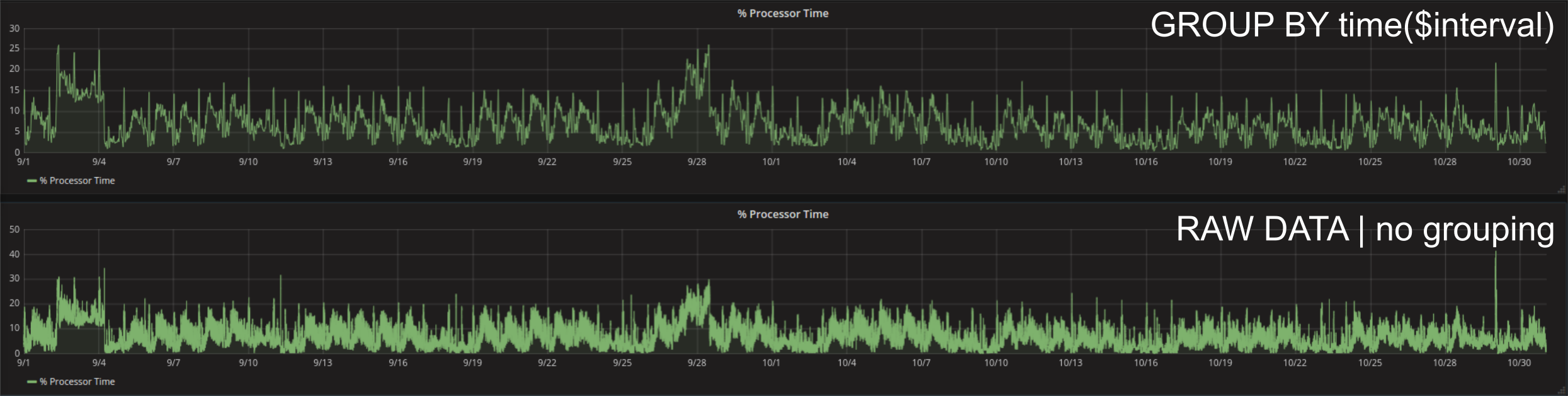
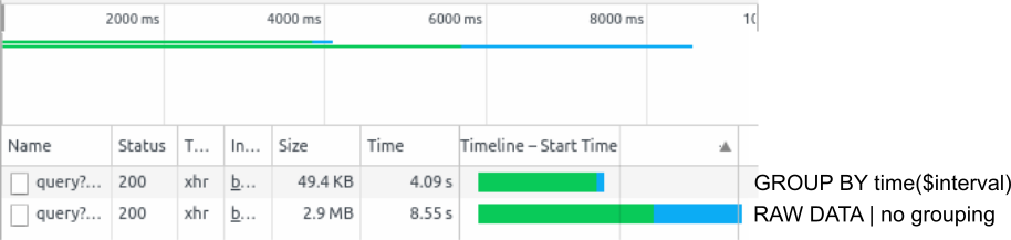
One of the easiest ways to analyse the time that a query needs is via the Chrome DevTools. These can be opened by pressing F12 while navigating with Chrome browser. A refresh of the dashboard with open DevTools shows the order and duration of each query and also the amount of data that is needed to be transferred. For example two months of processor time data loaded with the auto grouping can result in approximately 30m precision. In other words, the mean of the values is asked to data groups (30m of data each) and only the result is transferred from the underlying database to Grafana (49,4KB). Raw data can be queried by not using any grouping. In that case every single datapoint within the database(e.g. 2s precision => 30 x 60 x 24 x 61 = 2635200 datapoints: 2.9MB).
USE UNITS AND TRANSFORMATIONS
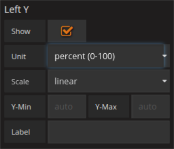
To make the shown results more interpretable, Grafana offers the possibility to specify the unit of the time series one is visualizing. This can also be separately for up to two y-axes in the axis menu.
A transformation such as for example the moving average can be used to smooth the data and make trends easily visible. Moving average means that that a window of a certain length is shifted along the time series and the mean of all points falling within the window is taken and visualized. Single extreme peaks get flattened this way and large scale dynamics of the visualized curve become more apparent.
Only precaution that needs to be taken is that when doing a moving mean at a very low precision one needs to keep in mind that there will be a shift in the data (orange region). Why is this the case? Grafana (at least when combined with InfluxDB) only accepts a value for the window size that specifies the number of points that should be considered. The first moving mean can be calculated after that number of time points. In terms of time the window size x the grouping precision.
Let us make this clearer with an example:
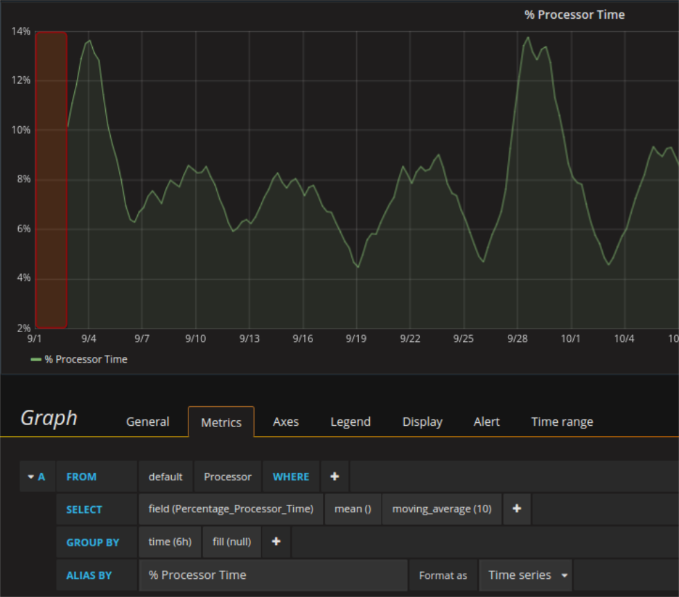
The query producing the graph in question has a grouping precision of 6h (it loads the mean value of all values of 6h from the database). Applying a moving average with window size 10 to the output means that 10 of the mean values are taken and the mean of the means is than calculated. This is possible for the first time when 10 mean values are available, so after 6h x 10 = 60h = 2.5d. Grafana depicts the obtained value not at the center of the window but at its end. The first value calculated is therefore shown at the timestamp 2.5 days after the beginning of the registration. The graph can be therefore seen as shifted to the right (an amount of 2.5d / 2 = 30h) and after zooming (when auto grouping precision changes) there position can be expected to change accordingly.
CONSIDER WHAT YOU REALLY WANT TO SHOW
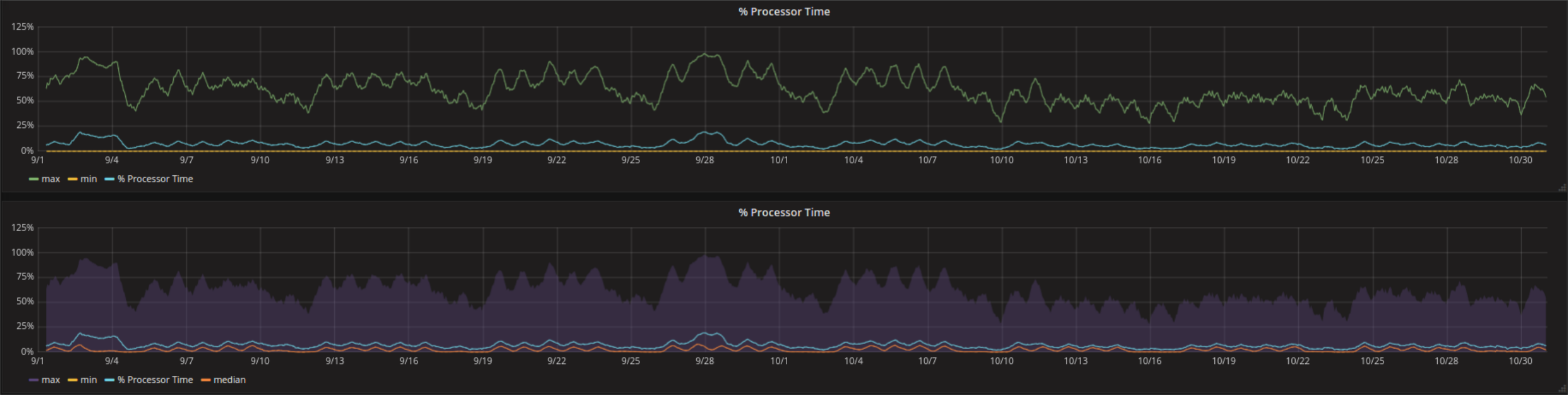
The (moving) average of a curve is one way to represent what happened during the time period of interest. For quite a few metrics the median or the range of the traffic during the time period of interest might even be more interesting. 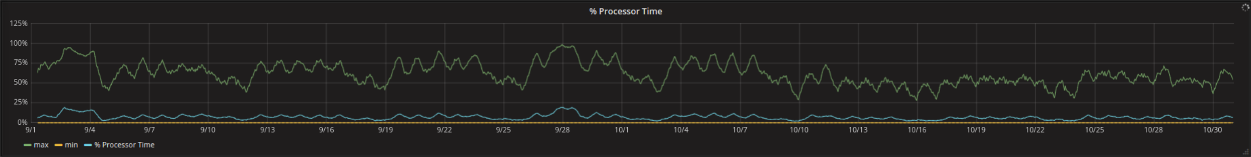
The relative queries could be as seen here:
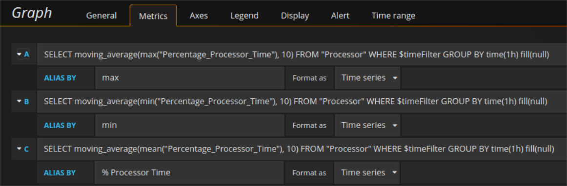
Too many similar curves within the same graph might look confounding. One way to deal with this is to keep the most relevant information as a line and transform the area between max and min values to a semitransparent range.
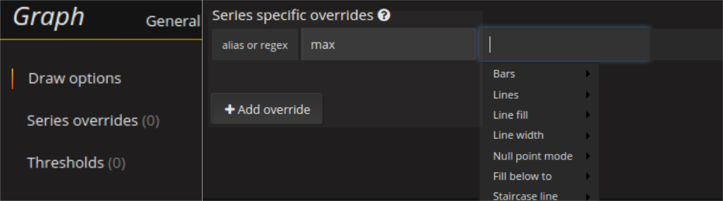
A visualization like this can be configured in the series specific overrides using the fill_below_to option and selecting lines as false for the lower curve of the range.
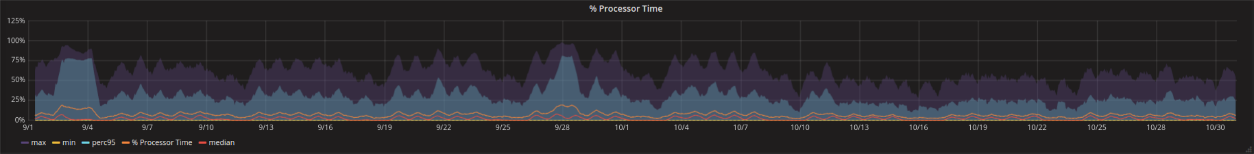
But do not exaggerate with such ranges, they are quite costly. Especially when using percentile instead of max or min the load time of the dashboards might increase notably and the output might not gain as much in quality.
OPTIMIZE DATA BASE CONTACT
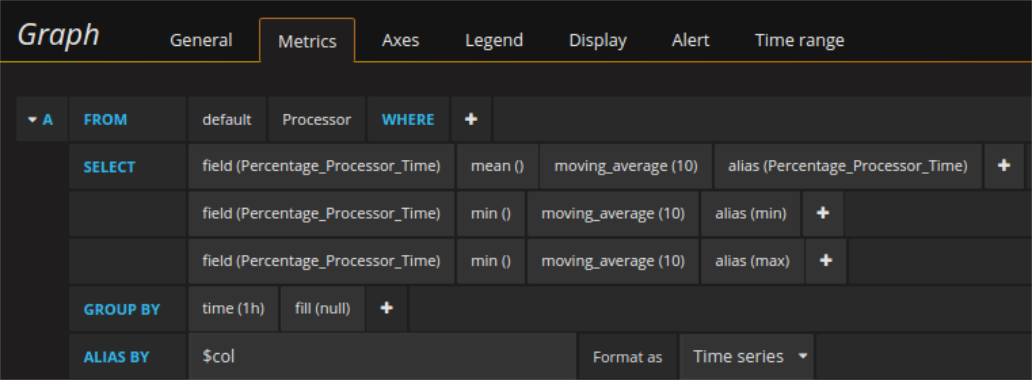
The same values can be retrieved in different ways from the database. For example the mean, the max, and the min can be queried by 3 single queries that return one column of data each or be formulated as a single query that gets three columns of data back from the data base. Even in the latter case aliasing is possible by assigning an alias to each field and putting $col into the alias field of the whole query. This way all series overrides work the same way as before. For small queries there might not be much difference, but 3 times a single column means also all the indexes/time stamps every time and data to transfer increase.
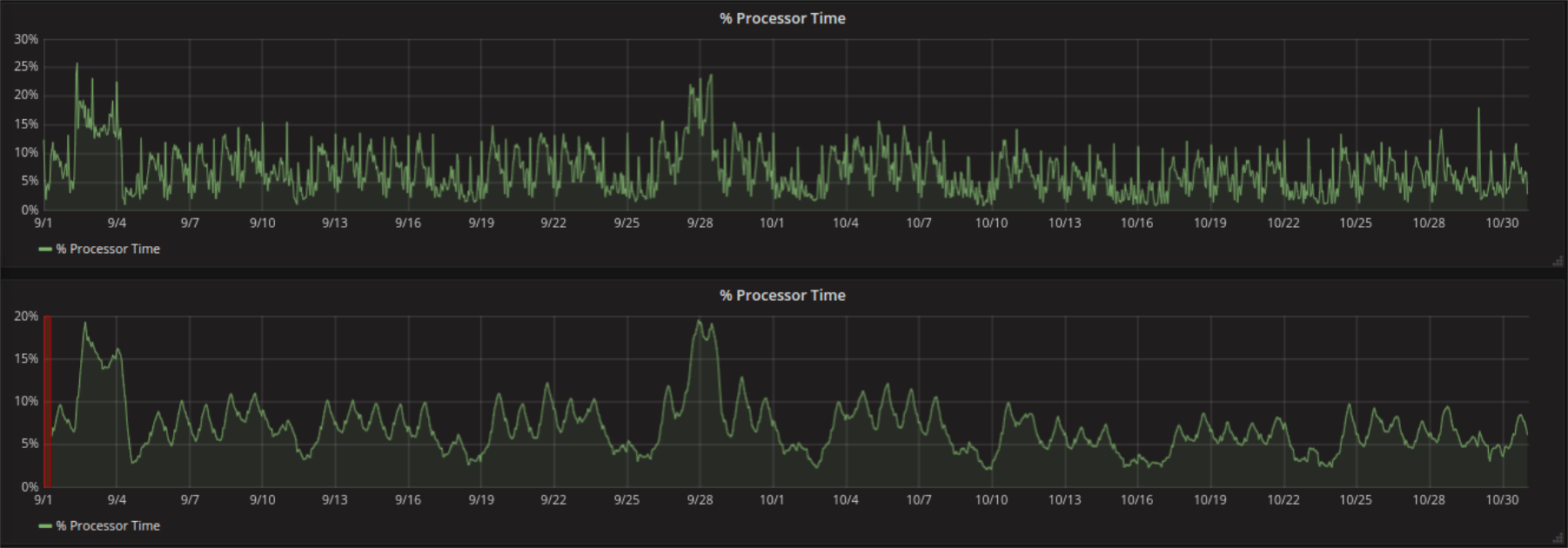
This gets especially relevant for example when performing the same query for multiple graphs of the dashboard. One use-case is the forced alignment of the y-limits of two dashboards. This is currently only possible by placing hard code limits (variables are not yet usable as limits) for the y-axes or by loading the data from one graph into the other respectively and to hide the not interesting one needed only for scaling. Let us make this clear by an example:
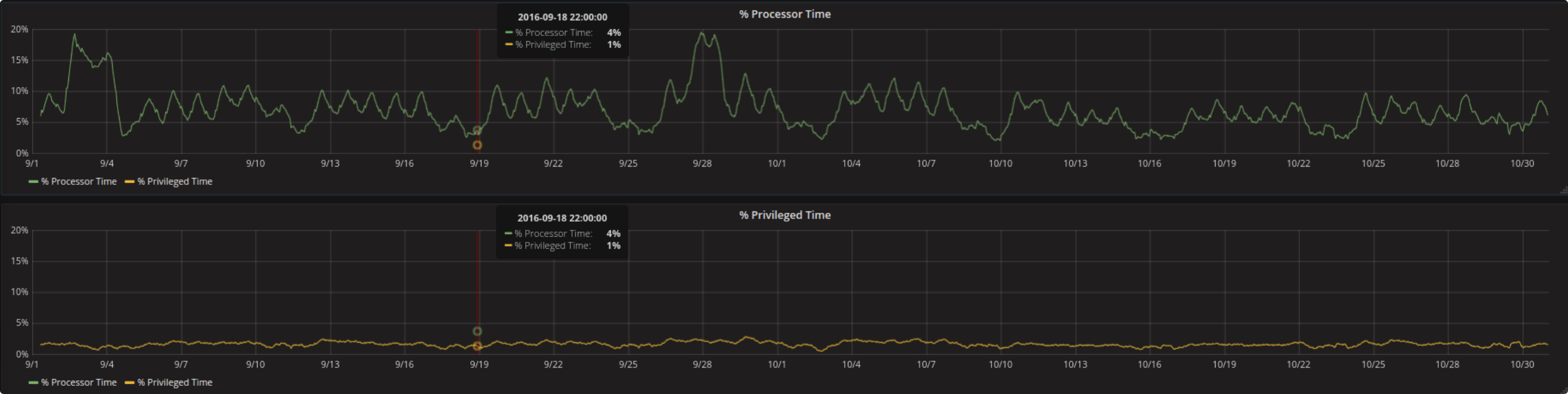
Percentage Processor Time and Percentage Privileged Time are both metrics from the same measurement (processor). To show them contemporaneously in two different graphs but with the same scaling on the y-axis one can load the respective other metric in a hidden way (set line width to 0, lines = false will make it disappear completely instead).
In such a setting (depending on the amount of data) it can happen that the first graph is blocking the loading of the second one especially when the queries are formulated as single ones as described above. With the help of the Chrome DevTools it is easy to spot such settings and to take a counteraction.
USE STEPWISE LOADING
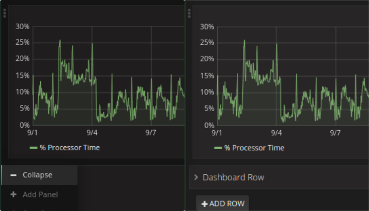
If you need many graphs, consider whether there are some more important than other. It is possible to organize them in groups (rows) and collapse some of them at the beginning. Collapsed rows will only be loaded when opened so you avoid slowdowns during the initial loading of the really relevant data that every user wants to see as fast as possible.
CONCLUSIONS
Always consider who is going to use your dashboards and the precision they really need. In case you cannot decide in favor of auto precision, consider a template variable for the grouping precision. This way you can speed up the initial loading. If the user really needs more precision he is able to get it in a second moment (when he hopefully is more prepared to wait). Use transformations and/or maths to get the visualization as close as possible to the curve a user is comfortable with.
Use DevTools to check the dynamics of the loading process of your dashboards.

Susanne Greiner
Hi there! My name is Susanne and I joined Würth-Phoenix early in 2015. Ever since I can remember computers and the perfection that can be reached by them have been very fascinating for me. I built my first personal PC using components from about 20 broken ones at the age of 11 and fell in love with open source, visualization and data analysis shortly afterwards. I hold a master in experimental physics (University of Erlangen, Germany) and a PhD in computer science (Universtiy of Trento, Italy) my main interests are machine learning, visualization techniques, statistics and optimization. As long as an algorithm of mine runs at night and I get new interesting results the morning after I am able to sleep well. Beside computers I also like music, inline skating, and skiing.
Author
Latest posts by Susanne Greiner
21. 09. 2018
NetEye, Service Management
HackTheAlps Challenge with Würth Phoenix
04. 04. 2018
Anomaly Detection, Events, ITOA, NetEye
Würth Phoenix @ GrafanaConEu 2018
27. 03. 2018
Anomaly Detection, ITOA, NetEye, Visual Synthetic Monitoring
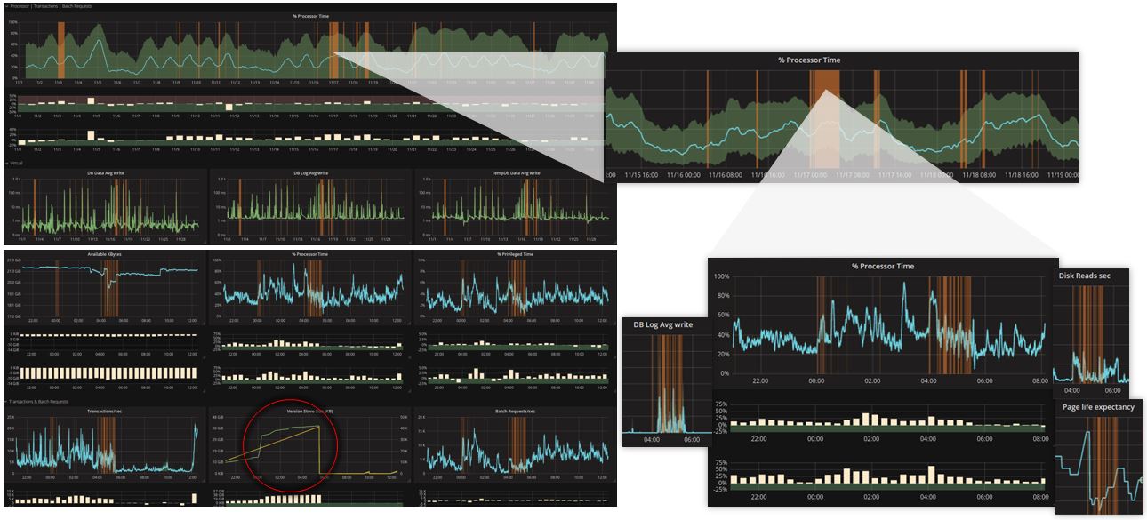
Multi-Level Dashboarding with Grafana – Use Case: NetEye ITOA | Alyvix
how to change the row title on grafana dashboard to lowercase ..by default its coming in Capital letter .please suggest me the way to make it in camel case or lowercase
are you maybe still back at version 3.1.1 (in that case the row titles will always appear capitalized even if you write them in camel case o lower case)
by upgrading to 4.1.2 (most probably even 4.0) you solve, because this has been changed and the row titles will appear the same way you type them into the title field under row options (click on the left upper corner of the first dashboard contained in the row). Hope this helps!
Hi,
thanks a lot for this useful article. I struggled also with performance-issues, and grouping helps. However, if I want to inspect a certain timerange in detail, the grouping does not allow this.
Ideal would be, that the grouping itself would be variable, so e.g. group by 1 hour, if the visible time range is a month or so, but when you zoom in, the grouping gets finer, e.g. group by 1m, if the zoomed range is 12h…
Is something like that possible?
Ok, figured it out by myself: There is already the possibility to choose ‚$_interval‘ besides from fixed time settings, that is doing the job exactly like I wanted… 🙂